Routing · Machine learning · An experiment
From Hexagons to Driving Times
How much road-network detail do we need to estimate a drive?
Imagine a planner comparing thousands of possible pickups and drop-offs. Again and again, it needs the same kind of answer: how long would this drive take?
A routing engine can find the shortest journey for each pair. But could we do some of that work once, store a small description of the road network, and use it to estimate new trips?
That is the question behind this experiment. The idea is to divide a city into hexagons, choose a few representative road locations around each one, and precompute the driving durations between them. Then we can ask two questions: how accurately can we estimate a trip, and how much do we gain by making the hexagons smaller?
The story and findings come first. The technical appendix contains the exact sampling, features, routing details, and reproducibility notes. Code and results are on GitHub.
Give each hexagon a few familiar places
H3 provides a grid of geographic cells at different sizes. For each hexagon, I take its six vertices and snap them onto nearby roads. These road locations become its landmarks.
Before estimating any trips, I calculate the driving duration between every pair of landmarks. This gives us a table describing how different parts of the city connect. The table respects direction: A→B can take a different amount of time from B→A.
I tested three H3 resolutions: 6, 7, and 8. A higher number means smaller hexagons and more landmarks. Smaller cells should capture more local detail, but that detail has a cost: more landmark pairs to calculate and store.
First, build a journey through the landmarks
Suppose the pickup and drop-off are in different hexagons. We can construct a journey in three pieces: pickup to a landmark, landmark to landmark, and finally landmark to drop-off.
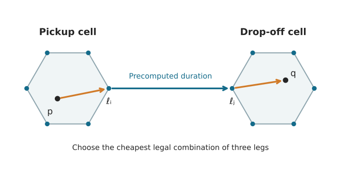
Each endpoint has six landmark choices, so there are 36 combinations to compare. Add the three durations for each combination and take the smallest total. This is our landmark dynamic-programming estimate, or DP.
The middle duration is already in the table. We still need to calculate the first and last legs. Plain single-source, multi-target Dijkstra can do that: one search from the pickup to its landmarks, and one from the drop-off on the reversed directed graph to obtain the landmark-to-drop-off durations. The experiment uses OSRM’s Contraction Hierarchies engine for these searches; the appendix explains the implementation.
There is a useful consequence of constructing a legal journey: it cannot be faster than the shortest possible journey. The DP estimate is an upper bound under the same routing model. We may force an unnecessary detour through a landmark, but we do not invent a faster route.
That pessimism can be valuable when underestimating a trip is costly—for example, when a planner needs to protect a pickup deadline. It is a guarantee about the static road model, though. Real traffic and service delays can still make the vehicle late.
Then, let a model use the same information
The landmark route can be an awkward detour. A nearby landmark might be on the wrong side of a major road, or simply in the opposite direction from the destination. A learned model has more freedom: it can use the landmarks as clues without requiring the journey to pass through them.
I give the model the 36 stored landmark-to-landmark durations, the positions of the endpoints relative to their landmarks, and the straight-line geometry of the trip. It predicts the whole duration directly. It does not need the exact endpoint routing legs used by DP.
I kept the comparison to three familiar approaches:
- Ridge regression: a simple linear combination of the features.
- Gradient-boosted trees: a model that can learn nonlinear rules and interactions.
- A small neural network, or MLP: another way to learn nonlinear relationships.
These models trade away DP’s guarantee. They can learn to remove an unnecessary landmark detour, but they can also underestimate the true shortest duration.
What happened in the three cities?
I ran the experiment in Tel Aviv–Gush Dan, Amsterdam, and the New York City area, training each city independently. All methods and resolutions use the same test trips, whose endpoints are held out from training.
The road patterns look quite different: Tel Aviv–Gush Dan mixes small grids and curving connectors, Amsterdam’s central streets bend around the city center, and Manhattan has a long, regular grid. These three views cover the same 12 × 12 km area.
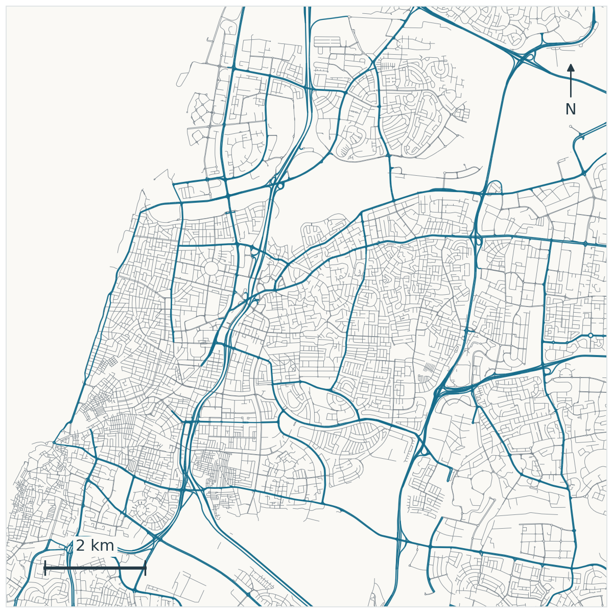
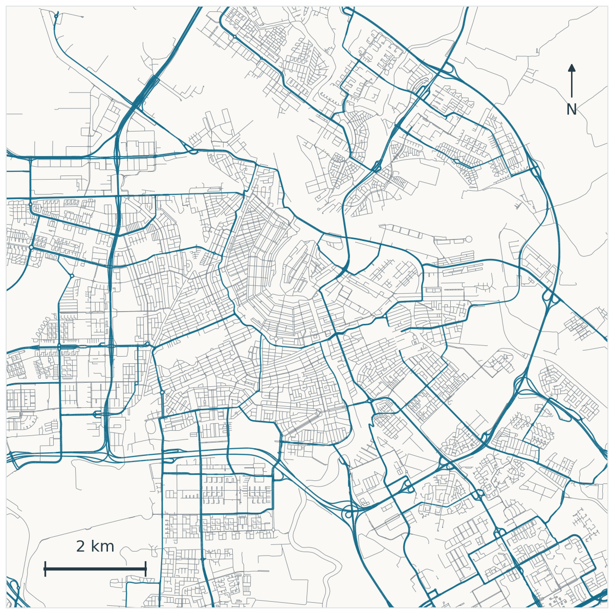
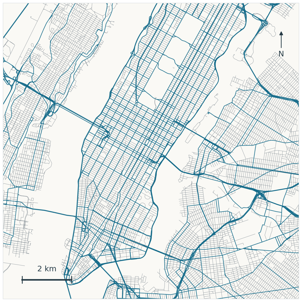
Same scale, north up. Major roads are blue; other streets are gray. These are cropped views within the study regions; full-region maps and drawing details are below. Tap a map to enlarge it. Map data © OpenStreetMap contributors.
The maps provide context for the experiment. They do not, by themselves, explain the differences in prediction error between cities.
Two boundaries matter when reading the results: “ground truth” means a shortest duration from a static router, with no traffic, and every tested trip crosses hexagon boundaries at all three resolutions. The trips are sampled from roads rather than actual ride demand. Same-cell journeys are outside this experiment.
The main measure is mean absolute error (MAE): the average size of the difference between an estimate and the router’s answer, in seconds. Smaller is better.
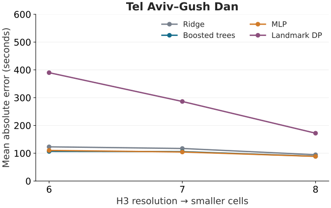
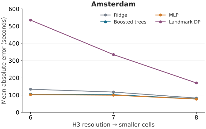
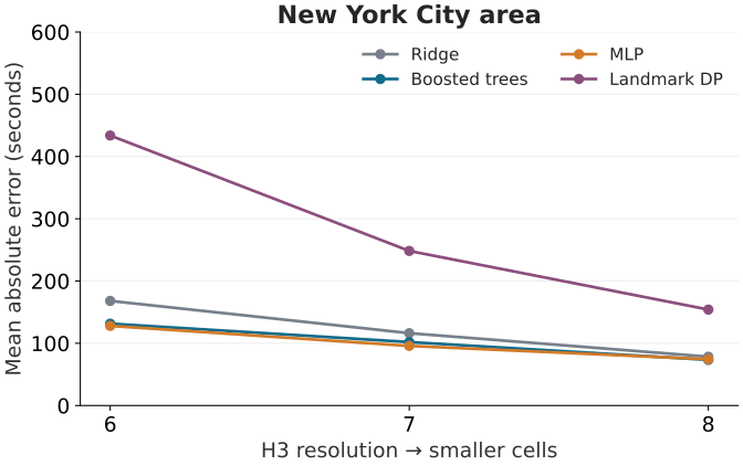
The pattern was consistent: finer cells improved every method, and the learned models had lower average error than DP. Here are the results at resolution 8, the finest grid tested:
| City | Ridge | Boosted trees | MLP | DP |
|---|---|---|---|---|
| Tel Aviv | 94.5 | 89.1 | 88.6 | 172.1 |
| Amsterdam | 82.4 | 77.4 | 76.2 | 170.1 |
| NYC | 78.4 | 73.4 | 74.3 | 154.1 |
The MLP and boosted trees are very close. Their average errors are about 1.2–1.5 minutes, compared with roughly 2.6–2.9 minutes for DP. The MLP narrowly wins in two cities; boosted trees narrowly win in NYC. Those small differences, from one split, do not establish a reliable accuracy winner.
Ridge is worth noticing too. At the finer resolution, even a linear model is fairly competitive. We did not need an elaborate model to get a useful estimate from this representation.
Average error still leaves room for larger misses. For boosted trees at resolution 8, the 95th-percentile absolute error is about 3.4–4.4 minutes. That matters if a few bad underestimates can disrupt a schedule.
How much detail is worth storing?
The coarsest cells already retain useful information. At resolution 6, boosted trees achieve errors of about 106 seconds in Tel Aviv, 105 in Amsterdam, and 131 in NYC. Their landmark tables occupy only about 45 KB, 48 KB, and 250 KB.
Making the cells smaller improves accuracy, but the table grows quickly. Double the number of landmarks and the number of ordered landmark pairs quadruples.
NYC shows the tradeoff clearly. Moving from resolution 6 to 8 reduces boosted-tree MAE from 131.5 to 73.4 seconds—about a 44% improvement. The table grows from 0.25 MB to 127.5 MB, roughly 510 times larger.
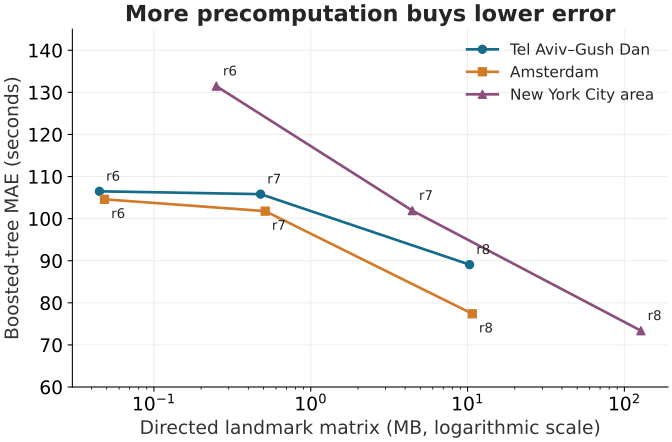
Resolution 7 offers an intermediate choice. In NYC, its table occupies 4.44 MB and the MLP has an average error of about 96 seconds. Resolution 8 brings that error down to about 74 seconds, with a 127.5 MB table. Whether those 22 seconds are worth the additional storage depends on the application.
These storage figures cover the landmark matrix. Trained models, landmark metadata, and any routing graph needed by the application take additional space.
What would I use?
My default from this experiment is the MLP at resolution 8, if the landmark table fits the memory budget. It was among the most accurate choices in every city and had lower measured individual-query latency than boosted trees.
Boosted trees at resolution 8 are an equally credible choice on accuracy. With a tighter memory budget, I would start at resolution 7 and check whether the additional error is acceptable. Resolution 6 is worth considering when the table must be very small.
I would choose DP when the static upper-bound guarantee is essential. Its higher average error buys a property that these regressors do not provide. The right choice depends on whether the application values a close estimate or needs protection against underestimation under the model.
The finding I take away is that a coarse representation can already support useful predictions on unseen endpoints within a city. More detail improves them, but the storage cost rises much faster than accuracy improves.
The next questions are practical ones: does this hold on real trip demand, including short journeys? How much do the landmark durations add beyond geometry alone? And can a model trained to penalize underestimation provide a useful compromise? Those are follow-up experiments; the results here do not answer them yet.
Technical appendix
This section records the choices behind the results. The main recommendation above is limited to this protocol and its sampled trips.
A. Data, ground truth, and splits
Ground truth is shortest driving duration on OpenStreetMap roads using a pinned OSRM 5.27.1 car profile configured to minimize duration. Traffic is ignored. These are router labels, not durations measured from actual vehicle trips. The map requests use the historical timestamp September 17, 2026.
Each study region is an explicit rectangle with a 0.12-degree routing buffer. The NYC rectangle includes nearby urban roads outside the city boundary. The buffer allows routes to leave the endpoint region, although sufficiently long detours can still be cut off.
For each city, I sample 3,000 endpoint locations approximately in proportion to eligible road-segment length. A position is drawn within the middle 90% of a selected segment and snapped within 100 metres. This gives broad road coverage; it does not reproduce the spatial distribution of ride requests.
The endpoints are split into three disjoint pools: 2,250 for training, 375 for validation, and 375 for testing. Unique directed pairs are sampled within each pool. A→B and B→A are different examples. No endpoint is shared across the three splits, although an endpoint can occur in multiple pairs within its own split.
A pair is accepted only if its endpoints belong to different cells at all three tested resolutions. This keeps the same pairs across resolutions and methods. It also means this experiment excludes many short trips and says nothing about same-cell accuracy. A practical same-cell routing fallback is possible, but it is not evaluated here.
The requested split sizes are 12,000 training pairs, 2,000 validation pairs, and 2,000 test pairs. After excluding unreachable or zero-duration labels, the test sets contain 1,962 trips in Tel Aviv, 1,962 in Amsterdam, and 1,983 in NYC. Every method returns a finite estimate for every retained test pair.
The main metric is mean absolute error (MAE), in seconds. I also record the 95th percentile of absolute error and signed bias, defined as prediction minus ground truth. The experiment uses one fixed seed and split. Small differences between models should not be read as statistically established wins.
| Study region | Bounding box |
|---|---|
| Tel Aviv–Gush Dan | [34.72, 31.95, 34.95, 32.22] |
| Amsterdam | [4.72, 52.28, 5.05, 52.44] |
| New York City study rectangle | [-74.26, 40.49, -73.7, 40.92] |
Protocol: duration_approximation_v6. Random seed: 20260918. Map request timestamp: 2026-09-17T00:00:00Z. These rectangles define the endpoint regions; the routing extract includes the additional buffer described above.
Road-map illustrations
These maps show the full endpoint study rectangles. The orange outline marks the 12 × 12 km window used in the main article. The full regions have different sizes, so these overview panels have different map scales; each has its own scale bar.
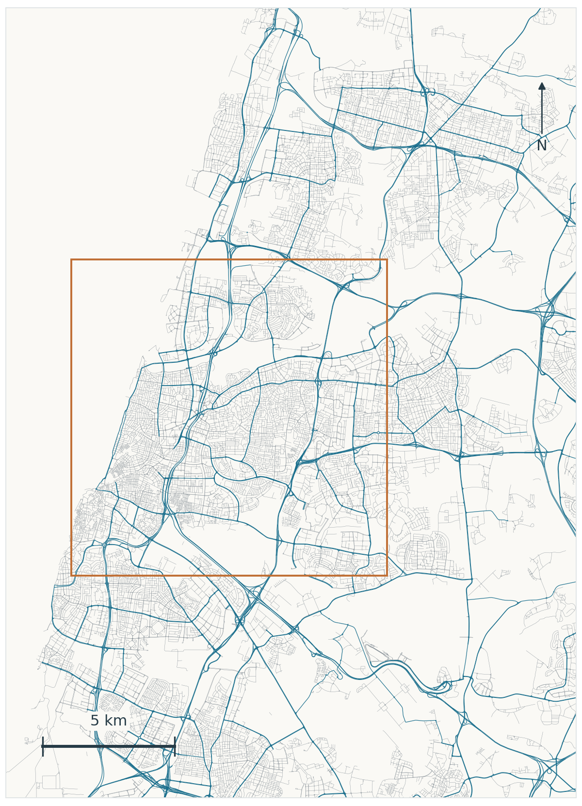
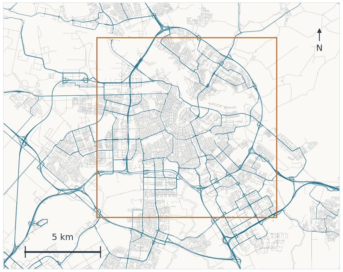
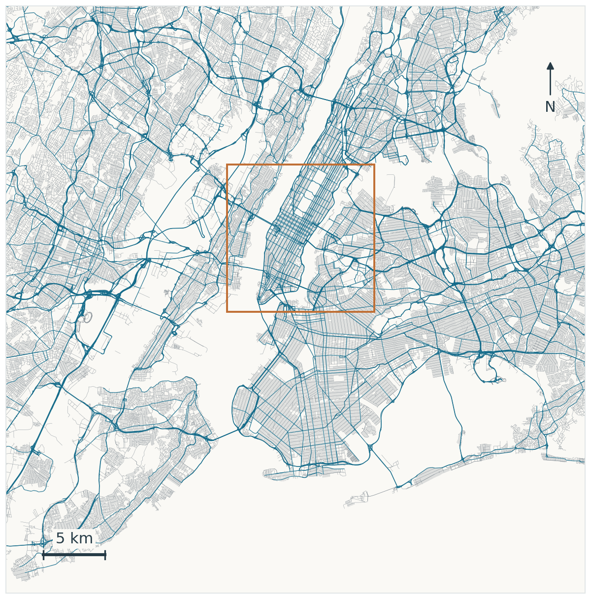
Full study regions, north up. Orange: the equal-size comparison window. Map data © OpenStreetMap contributors, ODbL 1.0.
The illustrations use separate OpenStreetMap geometry queries at the protocol’s historical timestamp, 2026-09-17T00:00:00Z. They are cartographic extracts, not the byte-identical frozen OSRM extracts used to produce the experiment’s labels. No experiments were rerun to make these figures.
Displayed road classes are motorway, trunk, primary, secondary, tertiary and their link roads, plus unclassified, residential and living streets. Service roads are omitted for clarity. Blue denotes motorway through secondary classes and their links; the remaining displayed streets are gray. Access rules, driving directions, turn restrictions and water polygons are not drawn. Blank areas therefore do not necessarily indicate water, and the pictures are not a complete representation of the routable graph.
Coordinates are drawn in a local equirectangular projection, scaling longitude by the cosine of each view’s center latitude. The comparison windows are centered at longitude/latitude (34.81, 32.08), (4.9, 52.365), and (−73.975, 40.75). The GitHub repository includes the compressed geometry, exact queries, source and geometry checksums, and the map drawing script. The same geometry produces both the cropped and full-region views.
B. Landmarks, routing, and the DP bound
H3 assigns geographic coordinates to cells at different resolutions. Higher resolutions mean smaller cells. I used resolutions 6, 7, and 8; their global average hexagon areas are approximately 36.1, 5.16, and 0.737 km². Individual cells vary in size. See the H3 resolution table.
For each cell, its six vertices suggest six representative places. A geometric vertex might fall in a building or a canal, so it must be snapped onto the road network. In this experiment, a landmark is the nearest eligible road position with one fixed legal driving direction. It can sit partway along a road segment; it is not necessarily an intersection. Shared vertices and identical snapped directed positions are deduplicated.
Direction matters. A road position approached from the north is not always interchangeable with the same position approached from the south. Treating them as identical can accidentally join two individually valid route segments into an invalid journey.
For every ordered pair of landmarks, I store the shortest driving duration. The matrix is directed: driving from A to B can take a different amount of time from driving from B to A. With L unique landmarks, a dense float32 table takes 4L² bytes. This implementation stores the complete matrix, including diagonal and within-cell entries.
The grid coverage follows road geometry sampled every 100 metres, plus a one-cell ring. It covers the study region before trip sampling is evaluated; it is not built only around the test pickups.
Let p and q be the pickup and drop-off, ℓᵢ a pickup-cell landmark, and ℓⱼ a drop-off-cell landmark. Write d for exact shortest driving duration and Mij for the precomputed duration from ℓᵢ to ℓⱼ. The estimate is:
This is a small dynamic program over three layers. We can minimize over the destination landmarks for each origin landmark, then take the minimum over origins. With only 36 combinations, a direct array minimum is sufficient. There is no need to run another general shortest-path algorithm over these layers.
The middle leg is a lookup. The first and last legs still require exact routing at query time. A straightforward implementation can use plain Dijkstra with one source and multiple targets on a routing graph that represents legal driving movements:
- Run Dijkstra from the pickup, targeting all of its cell’s landmarks.
- Run Dijkstra from the drop-off on the reversed directed graph, targeting all of its cell’s landmarks. These distances give the required landmark-to-drop-off durations in the original graph.
Each search can stop when every target landmark has been settled (its shortest distance finalized), or when the search queue is empty. This gives the endpoint legs with two single-source, multi-target searches.
In this experiment, those legs are computed through two local OSRM table requests using its Contraction Hierarchies routing engine. Plain Dijkstra is an alternative implementation of the same shortest-path calculations, not the engine used for the reported timings. The searches are not restricted to the endpoint cells. DP therefore retains an online routing dependency.
Why the bound holds
Every feasible combination describes a legal journey. The shortest possible journey cannot be longer than one of those journeys. Therefore, with compatible directed landmark states and the same routing costs, T̂(p, q) ≥ d(p, q). Taking the best landmark combination preserves the upper bound.
This is a useful kind of pessimism. If underestimating duration is much worse than overestimating it—for example, when a planner must protect a hard pickup deadline—a conservative estimate can be preferable to one with lower average error.
The guarantee is about the routing model. It does not guarantee arrival on time in the real world: traffic, uncertain speeds, and service delays are outside this experiment. Floating-point storage and OSRM’s rounded durations also require a small numerical tolerance when checking the bound.
Trip endpoints retain both legal driving directions where available, and routing minimizes over their explicit direction states. Intermediate landmarks keep one fixed legal direction so that route legs can be joined consistently. Numerical validation allows 0.31 seconds for a three-leg sum, accounting for decisecond rounding and float32 storage; direct route/table consistency uses a 0.11-second tolerance.
C. Features and model selection
Each example has 63 base features:
- 36 driving durations: every directed combination from the pickup cell’s six landmarks to the drop-off cell’s six landmarks.
- 24 local offsets: east and north displacement between each endpoint and each of its six snapped landmarks.
- 3 trip geometry features: pickup-to-drop-off east displacement, north displacement, and straight-line distance.
The duration block describes how the network connects the two areas. The offsets describe where the actual endpoints sit relative to those representative locations. The models receive neither absolute coordinates nor exact endpoint-leg durations.
I kept the model comparison deliberately small:
- Ridge regression: a regularized linear baseline. It asks how much we can achieve by combining these features with a weighted sum.
- Gradient-boosted trees: histogram gradient boosting, which can learn nonlinear thresholds and feature interactions.
- A small neural network: an MLP with hidden layers of 128 and 64 units, giving a different way to learn nonlinear relationships.
There are two predefined hyperparameter candidates per model family, selected by validation MAE. MLP epoch selection also uses validation data. Missing durations are imputed, with missingness flags; preprocessing and target scaling are fitted only on training data. Predictions are clipped at zero. Each city and resolution gets its own fitted models.
This is a comparison of three practical model families, not an exhaustive search for the best possible predictor. The exact settings are in the frozen protocol.
The fixed candidates and training settings are:
- Ridge: regularization
alphaof 1 or 100. - Histogram gradient boosting: 15 or 31 maximum leaf nodes; 250 iterations; learning rate 0.05; L2 regularization 1.0; automatic early stopping disabled.
- MLP: hidden layers (128, 64);
alphaof 0.0001 or 0.01; initial learning rate 0.001; batches of up to 256; at most 150 epochs, with validation patience of 15 epochs and the best validation epoch retained.
Nonfinite feature values become missing values. Median imputation adds missingness indicators, followed by feature standardization. All three models also use training-only target standardization. Hyperparameter candidates are selected by validation MAE; no additional model families or candidate settings were searched after inspecting test performance.
D. Full curves, error tails, and costs
Resolution-8 error tails and signed bias for boosted trees and DP, in seconds:
| City | Method | MAE | 95th percentile | Bias |
|---|---|---|---|---|
| Tel Aviv | Boosted trees | 89.1 | 264.4 | -7.0 |
| Tel Aviv | DP | 172.1 | 467.2 | +172.1 |
| Amsterdam | Boosted trees | 77.4 | 201.8 | -8.4 |
| Amsterdam | DP | 170.1 | 411.2 | +170.1 |
| NYC | Boosted trees | 73.4 | 209.6 | -4.7 |
| NYC | DP | 154.1 | 330.1 | +154.1 |
For boosted trees, the 95th-percentile absolute error is roughly 3.4–4.4 minutes. A near-zero mean bias would not imply that underestimation is rare; positive and negative errors can cancel. DP’s positive bias, by contrast, is almost identical to its MAE because its error is one-sided, apart from numerical rounding. Its conservatism comes with a substantial accuracy cost.
A finer grid creates more landmarks, and the all-pairs table grows quadratically in their number. The numbers below are the actual matrix payload, in decimal MB; they exclude the road graph, landmark metadata, and trained models.
| City | H3 | Landmarks | Matrix MB | Matrix time |
|---|---|---|---|---|
| Tel Aviv | 6 | 106 | 0.045 | 0.07 s |
| Tel Aviv | 7 | 346 | 0.479 | 0.51 s |
| Tel Aviv | 8 | 1,605 | 10.304 | 9.78 s |
| Amsterdam | 6 | 110 | 0.048 | 0.06 s |
| Amsterdam | 7 | 358 | 0.513 | 0.49 s |
| Amsterdam | 8 | 1,637 | 10.719 | 9.34 s |
| NYC | 6 | 250 | 0.250 | 0.59 s |
| NYC | 7 | 1,054 | 4.444 | 10.00 s |
| NYC | 8 | 5,646 | 127.509 | 268.90 s |
The full run used one CPU and 2 GiB of RAM, without a GPU. Mean individual-query times were roughly 0.7–0.9 ms for ridge and the MLP, 2.5–2.6 ms for boosted trees, and 4.0–6.9 ms for DP. ML timings include feature construction and inference; DP timings include its two local HTTP table calls. Common endpoint snapping is excluded. These are measurements of this implementation, not a claim about pure algorithm speed or a speedup over an optimized batched router.
There are clear limits to the evidence: one split, three independently trained cities, synthetic road-length sampling, cross-cell trips only, and static router labels. The experiment does not establish performance on real demand, traffic, unseen cities, or same-cell trips. It also has no geometry-only ablation, so it does not isolate how much improvement comes specifically from the landmark durations.
E. Reproduce the figures or the experiment
The standalone repository contains the frozen protocol, core experiment code, Docker runner, tests, all 36 result summaries, and this article’s figure generator. The published core modules are byte-identical to those used in the completed full run; a manifest records their hashes. No private service or credentials are needed to run the experiment.
The full run passed the DP bound check on every retained test prediction and 450 additional checks comparing selected three-leg journeys with joined waypoint routes. The standalone test suite has 15 tests. These checks are particularly important for direction handling: a fast estimate is not useful if its claimed bound comes from incompatible route legs.
The small result summaries are included in Git. Full per-trip datasets, model files, routing-map extracts, and landmark matrices are produced by the runner and are not bundled with this article. The separate geometry used only for the road-map illustrations is included in the repository. Reproducing the exact labels requires identical map bytes, not just the same timestamp; the runner records map identities and supports reuse of frozen extracts.
Map data © OpenStreetMap contributors, available under ODbL. Routing uses OSRM 5.27.1; models use scikit-learn 1.5.2. Protocol: duration_approximation_v6; seed: 20260918.